
Text representation I.
M.Sc course, University of Debrecen, Department of Data Science and Visualization, 2024
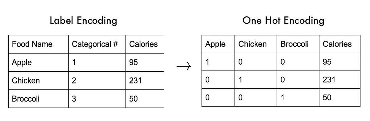
One-Hot
One-hot encoding is a technique used in machine learning and natural language processing to represent categorical data, such as words, in a binary format. In one-hot encoding, each category is represented by a binary vector where all elements are zero except for one element, which is set to one to indicate the presence of that category.
Here’s how it works:
- Define Categories: First, you need to define the categories that you want to encode. For example, if you’re encoding words in a vocabulary, each unique word would be a category.
- Create Binary Vectors: For each category, create a binary vector with the length equal to the total number of categories.
- Assign Values: Set the value of the element corresponding to the category to 1, and all other elements to 0.
For example, suppose you have a vocabulary of three words: “apple”, “banana”, and “orange”. You can represent each of these words using one-hot encoding as follows:
- “apple”: [1, 0, 0]
- “banana”: [0, 1, 0]
- “orange”: [0, 0, 1]
One-hot encoding is commonly used as a preprocessing step in machine learning models, especially in tasks where the input data is categorical and needs to be converted into a numerical format understandable by the algorithms. However, it has some limitations, such as high dimensionality and the inability to capture relationships between categories.
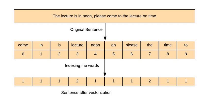
Counter Vectorization
Counter vectorization, often referred to as CountVectorizer, is a technique used in natural language processing (NLP) to convert a collection of text documents into a matrix of token counts. In simpler terms, it’s a method to transform a set of text data into numerical form so that it can be used as input for machine learning algorithms.
Here’s how counter vectorization typically works:
- Tokenization: First, the text data is tokenized, which means breaking it down into individual words or terms. This step may also involve removing punctuation, converting text to lowercase, and other preprocessing tasks.
- Vocabulary Building: Next, a vocabulary of all unique tokens (words or terms) across the entire corpus (collection of documents) is constructed. Each unique token is assigned an index in the vocabulary.
- Counting Occurrences: For each document in the corpus, the count of each token in the vocabulary is calculated. This results in a numerical representation of each document where each element represents the frequency of a particular token in the document.
- Vectorization: Finally, these counts are arranged into a matrix, where each row corresponds to a document and each column corresponds to a token in the vocabulary. This matrix is often sparse, meaning that most of its elements are zeros, since not all tokens appear in every document.
Counter vectorization is a fundamental step in many NLP tasks, such as text classification, sentiment analysis, and document clustering. While it provides a simple and efficient way to represent text data, it doesn’t capture semantic meaning or word relationships, and it can be sensitive to the size of the vocabulary and the frequency of tokens. Despite its limitations, counter vectorization is widely used and serves as a baseline for more advanced techniques in NLP.
TF-IDF
TF-IDF (Term Frequency-Inverse Document Frequency) is not a tokenization technique per se, but rather a weighting scheme used in information retrieval and text mining to represent the importance of words or terms in a document corpus. However, it is often associated with tokenization because it operates on tokens extracted from text.
Here’s how TF-IDF works in the context of tokenization and text analysis:
- Tokenization: The text data is first tokenized, breaking it down into individual words or terms. This step can involve various tokenization techniques, such as word-level tokenization or subword tokenization.
- Term Frequency (TF): For each term (token) in a document, the term frequency (TF) is calculated, representing the frequency of occurrence of the term in the document. TF is usually normalized to prevent bias towards longer documents. It can be calculated as:
- TF(term, document) = (Number of times term appears in document) / (Total number of terms in document)
- Inverse Document Frequency (IDF): IDF measures the importance of a term across the entire document corpus. Terms that are rare across the corpus but common within a specific document are given higher weights. IDF is calculated as:
- IDF(term) = log((Total number of documents) / (Number of documents containing term))
- TF-IDF Weighting: Finally, the TF-IDF weight of a term in a document is calculated by multiplying its term frequency (TF) by its inverse document frequency (IDF):
- TF-IDF(term, document) = TF(term, document) * IDF(term)
Representation: The resulting TF-IDF weights for each term in each document form a vector representation of the documents in the corpus. This representation can be used for various text mining tasks, such as information retrieval, document classification, and clustering.
TF-IDF tokenization, if we consider it as a process, involves tokenization followed by the calculation of TF-IDF weights for each term in each document. It allows for capturing the importance of terms in documents relative to the entire corpus, enabling more effective text analysis and information retrieval. TF-IDF is widely used in various NLP and text mining applications due to its simplicity and effectiveness in representing the significance of terms in text data.
Embedding
Word embeddings are dense vector representations of words in a continuous vector space, typically learned from large text corpora using techniques like Word2Vec, GloVe, or FastText. These embeddings capture semantic and syntactic similarities between words, enabling algorithms to understand and process natural language more effectively.
Here’s how the process of “embedding tokenization” might work:
- Tokenization: The input text is tokenized into individual words or subword units using a tokenization technique such as word-level tokenization, subword tokenization (e.g., Byte-Pair Encoding), or character-level tokenization.
- Word Embedding Generation: Each token (word or subword) is mapped to its corresponding word embedding vector in a pre-trained embedding space. This mapping is based on a learned embedding model trained on a large corpus of text data. The embedding vectors capture semantic and syntactic relationships between words, such that similar words have similar vector representations.
- Representation: The resulting embedding vectors form a dense representation of the input text, where each token is represented by a high-dimensional vector in the embedding space. These embeddings can then be used as features for downstream NLP tasks, such as text classification, sentiment analysis, or machine translation.
Embedding tokenization, as described above, combines tokenization with the generation of word embeddings to represent text data in a continuous vector space. This approach allows for capturing semantic meaning and contextual information from the text, enabling more sophisticated and accurate NLP models and applications.